Mci detection using fmri time series embeddings of recurrence plots
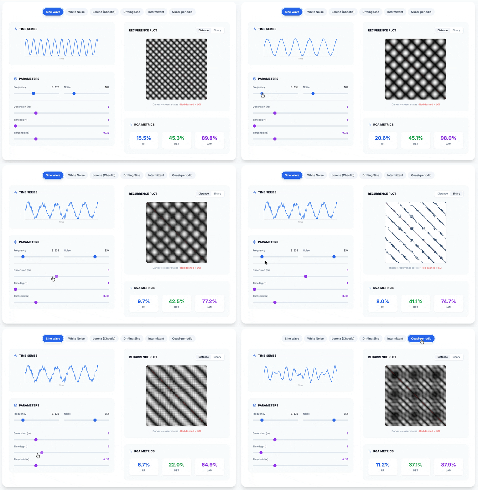
Originally introduced in non‑linear dynamical systems analysis, recurrence plots are a simple idea: take a time series, compare every time point with every other time point, and visualize similarity as a 2‑D image. What emerges is not noise, but texture — diagonals, blocks, disruptions — signatures of how a system evolves in time.
For brain signals, those textures are surprisingly informative.
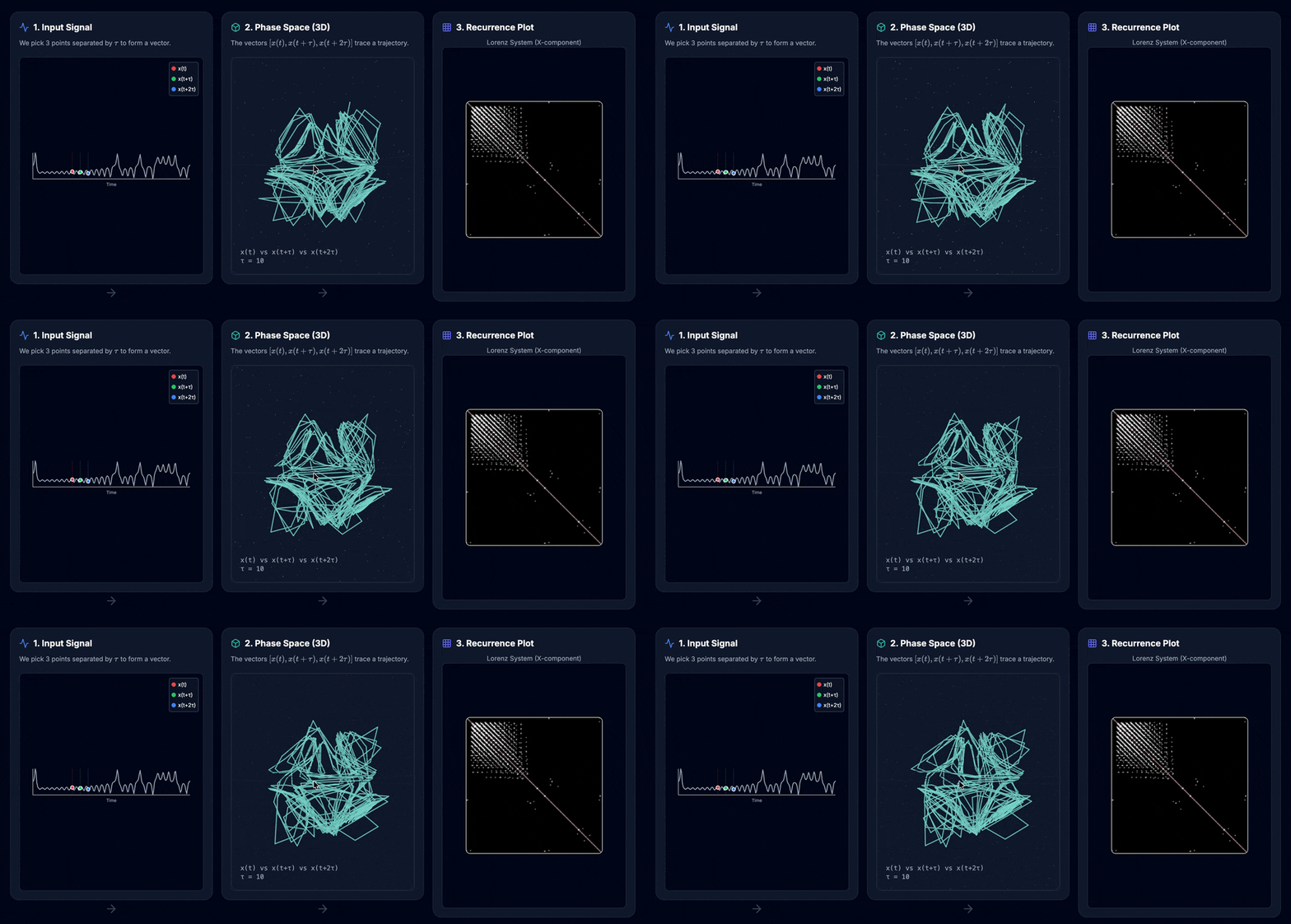
A resting‑state fMRI time series can be thought of as a trajectory through a high‑dimensional state space. Traditional pipelines collapse this trajectory into averages or pairwise correlations, implicitly assuming stationarity. Recurrence plots do the opposite: they preserve temporal organization by asking a single question repeatedly — has the system been here before?
When applied to neural data, the resulting images capture repeating motifs, regime shifts, and long‑range dependencies that are difficult to express numerically but easy to see.
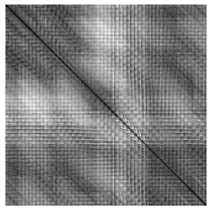
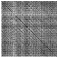
Even without labels, recurrence plots from healthy controls and subjects with Mild Cognitive Impairment (MCI) often differ in global organization. The distinction is not a single feature, but a redistribution of structure — diagonals fragment, blocks weaken, and regularity gives way to irregular recurrence.
Classical Recurrence Quantification Analysis (RQA) attempts to summarize these images using scalar descriptors: recurrence rate, determinism, laminarity, entropy. While useful, this compression is severe. Much of the spatial information that defines the plot’s character is discarded, and performance becomes sensitive to thresholding and parameter choices.
Rather than asking which scalar best explains disease, we instead ask a different question: can a model learn the representation directly from the recurrence structure itself?
Treating recurrence plots as images allows us to bypass handcrafted descriptors entirely. Convolutional neural networks and autoencoders can be trained to extract low‑dimensional latent embeddings that preserve the global geometry of the plot.
These embeddings act as compact signatures of neural dynamics. Importantly, they are learned, not imposed — the model discovers which spatial arrangements of recurrence matter for discrimination.
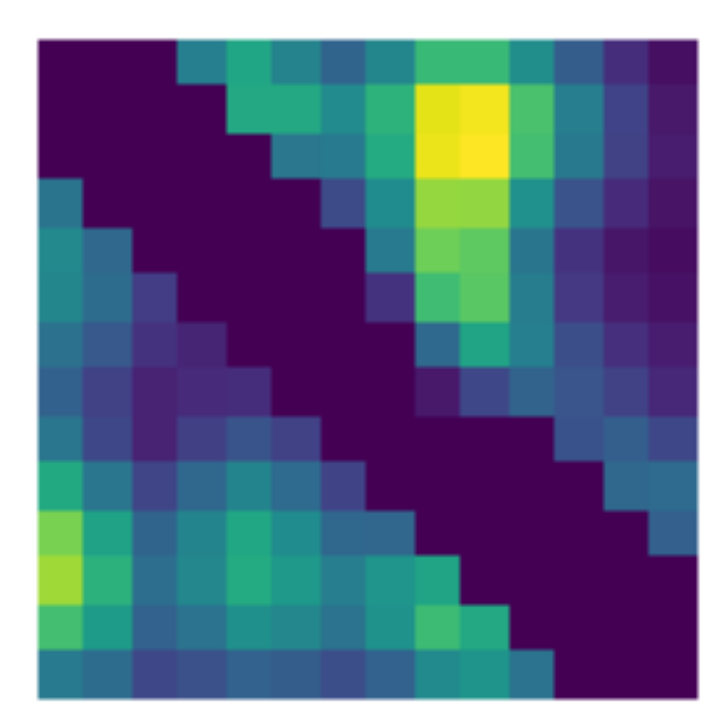
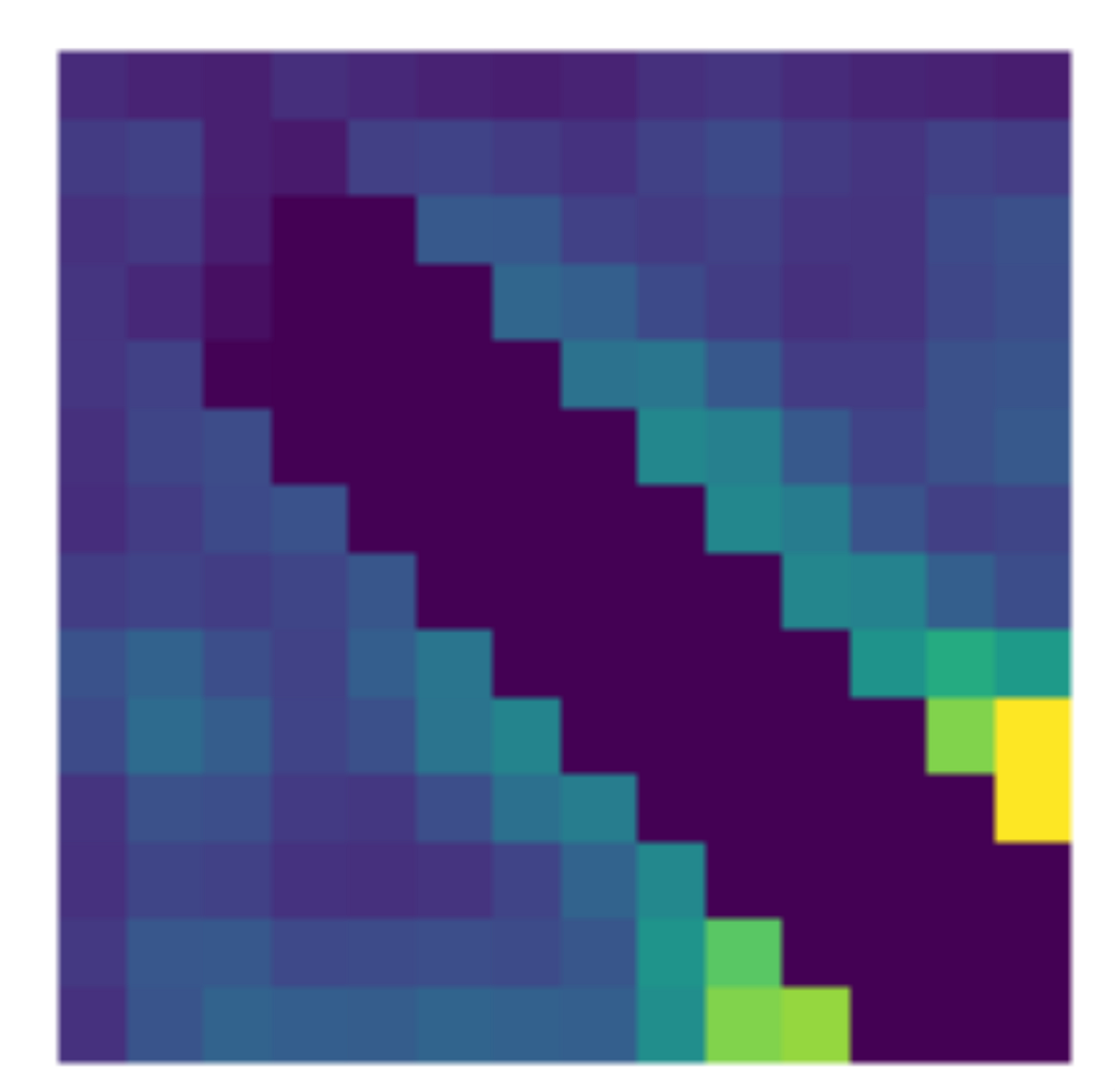
Across experiments, embeddings derived from recurrence plots consistently separate MCI from healthy controls more clearly than classical RQA features, even when trained on the same underlying time series.
A minimal construction
At a practical level, generating a recurrence plot requires little machinery. Given a multivariate time series, pairwise distances between time points are computed and visualized as a square matrix:
from scipy.spatial.distance import pdist, squareform
import matplotlib.pyplot as plt

D = squareform(pdist(time_series))
plt.imshow(D)
plt.colorbar()
Despite its simplicity, this transformation fundamentally changes how the data can be modeled. Temporal dynamics become spatial patterns, and time‑series analysis becomes representation learning.
If you are interested in interactive recurrence plots, parameter tuning, and hands‑on experimentation, visit https://recurrence‑plots.github.io/